Tensor Parallelism PyTorch
Deep learning is getting bigger especially for Language Model, and the relationship between performance vs size already explained in kaplan2020scalinglawsneurallanguage,
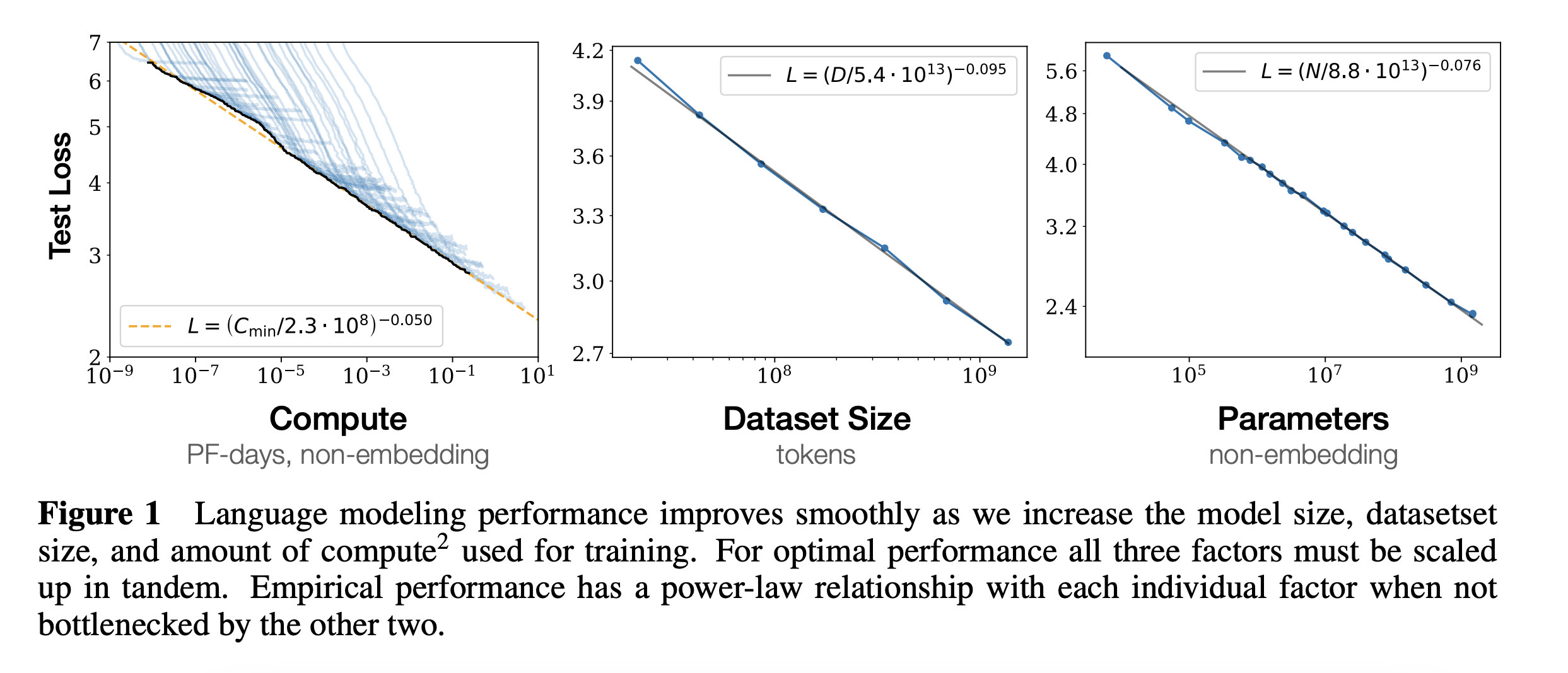
The more compute, more data, more parameters you have, the better the performance in term of perplexity.
And when GPT-3 released, which is 175B parameters, it changed the world. From the paper brown2020languagemodelsfewshotlearners, basically if you scaled large enough the parameters with the appropriate amount of dataset, the pretrained language model able to do any NLP task as long you give few examples or the technical term is few-shots learner, without need to go training session (training session in 2024 got multiple stages such as pretraining, continue pretraining, pre-finetuning, mid-finetuning, post-finetuning).
Now 175B is huge, the paper released in 2020, and 175B is insane even nowadays is still considered insanely large. GPT-3 trained on V100, mentioned in the paper section 2.3,
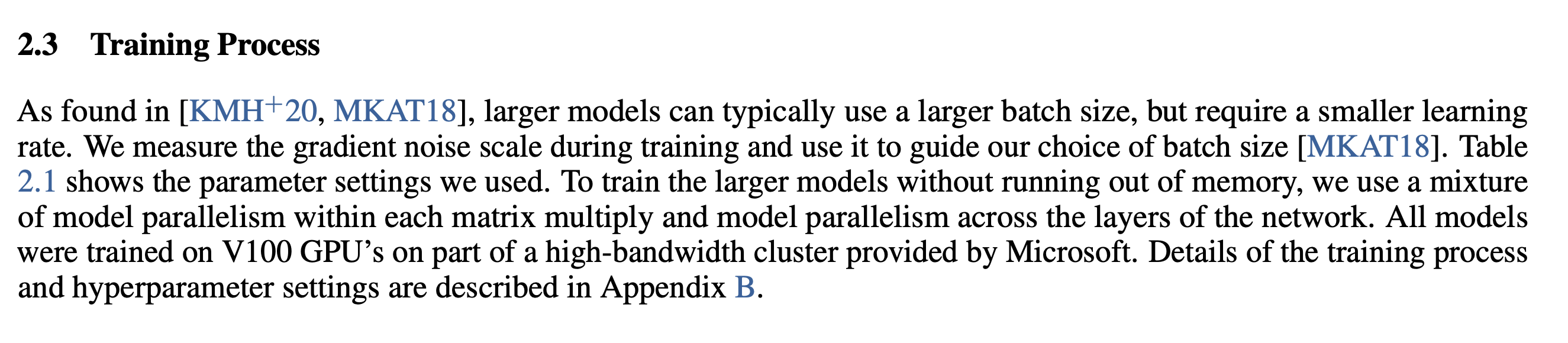
V100 is best for single-precision, which is 32 bit, assumed if the model saved in float32, 4 bytes, 175B * 4 bytes ~= 652 GB!
For V100, the biggest GPU memory is 32GB, 652GB / 32 = 21 GPUs! So you need at least 21 units of V100 32GB VRAM just to store the model in the memory, not yet feed-forward!
So how does OpenAI able to load the model into multiple GPUs? Tensor Parallelism!
As you can see, the model is not fit in a single GPU, so we have to shard the model. There are 2 sharding method for deep learning, 1. Tensor Parallelism, 2. Pipeline Parallelism.
Assumed I have a model with 2 hidden layers, 4x4 and 4x2, and 2 GPUs,
Tensor Parallelism shard hidden layers into multiple GPUs but all the GPUs got all the hidden layers. While Pipeline Parallelism split the hidden layers into multiple GPUs. Each method got their own pros and cons, but this blog we will look into Tensor Parallelism using PyTorch. And Tensor Parallelism itself got 2 different methods, 1. Row-Wise Parallel, 2. Column-Wise Parallel.
Row-Wise Parallel we shard the hidden layer in the row manner while Column-Wise we shard the hidden layer in the column manner.
Row-Wise Parallel
By using the same hidden layers size above,
- i. For the first hidden layer, we will split 4x4 into two row-wise and each GPUs store the weights, 2x4 GPU 0 and 2x4 GPU 1.
- ii. For the second hidden layer, we will split 4x2 into two row-wise and each GPUs store the weights, 2x2 GPU 0 and 2x2 GPU 1.
- iii. Input is 1x4 -> split into two column-wise and scatter to GPUs, 1x2 to GPU 0 and 1x2 to GPU 1, and each GPUs will do matmul, GPU 0 1x2 matmul 2x4 = 1x4, GPU 1 1x2 matmul 2x4 = 1x4, after that aggregate sum. In term of matmul coordinate,
- iv. Output from the first hidden layer now become the input, 1x4 -> split into two column-wise and scatter to GPUs, 1x2 to GPU 0 and 1x2 to GPU 1, and each GPUs will do matmul, GPU 0 1x2 matmul 2x2 = 1x2, GPU 1 1x2 matmul 2x2 = 1x2, after that aggregate sum. In term of matmul coordinate,
Column-Wise Parallel
By using the same hidden layers size as Row-Wise Parallel,
- i. For the first hidden layer, we will split 4x4 into two column-wise and each GPUs store the weights, 4x2 GPU 0 and 4x2 GPU 1.
- ii. For the second hidden layer, we will split 4x2 into two column-wise and each GPUs store the weights, 4x1 GPU 0 and 4x1 GPU 1.
- iii. Input is 1x4 -> replicated into the same as number of GPUs and scatter to GPUs, 1x4 to GPU 0 and 1x4 to GPU 1, and each GPUs will do matmul, GPU 0 1x4 matmul 4x2 = 1x2, GPU 1 1x4 matmul 4x2 = 1x2, after that aggregate concatenation. In term of matmul coordinate,
- iv. Output from the first hidden layer now become the input, 1x4 -> replicated into the same as number of GPUs and scatter to GPUs, 1x4 to GPU 0 and 1x4 to GPU 1, and each GPUs will do matmul, GPU 0 1x4 matmul 4x1 = 1x2, GPU 1 1x4 matmul 4x1 = 1x1, after that aggregate concatenation. In term of matmul coordinate,
Because you shard the weights into N devices, you save the memory for each devices by N size also! The more devices you have, the bigger model you can fit into.
So now, let us code Tensor Parallelism Row-Wise using PyTorch!
Why Row-Wise? because it looks harder, harder is good.
As we mentioned above, to do Tensor Parallelism, you must use multi-GPUs, and multi-GPUs required specific distributed communication, lucky in PyTorch, there are native interface to communicate in distributed manner, called Torch Distributed Elastic.
So what Torch Distributed Elastic do, each GPUs got it's own process,
- Let say I got 2 GPUs, Torch Distributed Elastic will spawn 2 processes, PID 0 for GPU 0, PID 1 for GPU 1.
- How does these processes communicated each other? Inter-process communication through open port. But for data transfer for deep learning model, if you are using Nvidia, by default it will use NCCL (pronounced as nickel) for gradients and weights synchronization.
- There are 3 important terms when talking about distributed system in Deep Learning framework or PyTorch, `RANK`, `WORLD_SIZE` and `LOCAL_WORD_SIZE`, `RANK` is the GPU rank, `WORLD_SIZE` is the total GPUs that you initialized and `LOCAL_WORLD_SIZE` is the total GPUs for each nodes if you are using multi-nodes. But if you are using a single node, `WORLD_SIZE` and `LOCAL_WORLD_SIZE` is same.
- GPU 0 is `RANK` 0 and GPU 1 is `RANK` 1, and `WORLD_SIZE` is 2. Both `RANK` and `WORLD_SIZE` able to fetch using OS environment variables which is automatically set by Torch Distributed Elastic.
- Assumed `RANK` 0 open port 29950 and `RANK` 1 open port 29951,
- NCCL is using their own communication called CUDA IPC, Inter-Process Communication, a peer-to-peer communication from devices to devices. Not all GPUs support P2P, so if not supported, NCCL will use an alternative such as shared memory located at `/dev/shm`.
- Why need different communications for multi-processing aka Torch Distributed Elastic and GPUs aka NCCL? Sockets or open ports use to check heartbeats and communicate simple strings among multi-processes while NCCL only designed for Nvidia Peer-to-Peer multi-GPUs communication.
Before we do Tensor Parallelism, let us try simple scatter and gather just to familiarize with PyTorch Distributed Elastic,
```python
import torch
import torch.nn as nn
import torch.distributed as dist
import os

def main():
    world_size = torch.cuda.device_count()
    local_rank = int(os.environ["LOCAL_RANK"])
    device = f'cuda:{local_rank}'
    dist.init_process_group(backend='nccl')

    tensor_size = 2

    output_tensor = torch.zeros(tensor_size, device=device)

    if dist.get_rank() == 0:
        t_ones = torch.ones(tensor_size, device=device)
        t_fives = torch.ones(tensor_size, device=device) * 5

        scatter_list = [t_ones, t_fives]
    else:
        scatter_list = None

    dist.scatter(output_tensor, scatter_list, src=0)

    print(f'local rank: {local_rank}', output_tensor)

    output_tensor += 1

    if dist.get_rank() == 0:
        t_ones1 = torch.ones(tensor_size, device=device)
        t_ones2 = torch.ones(tensor_size, device=device)
        scatter_list = [t_ones1, t_ones2]
    else:
        scatter_list = None

    dist.gather(output_tensor, scatter_list, dst=0)
    if dist.get_rank() == 0:
        print(scatter_list)

if __name__ == "__main__":
    main()
```
Save it as `simple-scatter-gather.py`, and this example originally from https://pytorch.org/docs/stable/distributed.html#torch.distributed.scatter, we just make it complete. This example required two GPUs, and to execute it using `torchrun`,
```bash
torchrun \
--nproc-per-node=2 \
simple-scatter-gather.py
```
And this CLI definition can read more at https://pytorch.org/docs/stable/elastic/run.html#stacked-single-node-multi-worker
```bash
torchrun \
--nproc-per-node=$NUM_TRAINERS \
YOUR_TRAINING_SCRIPT.py (--arg1 ... train script args...)
```
- `--nproc-per-node` is the size of GPUs you want to run, if set `--nproc-per-node=2` it will spawn 2 processes and each process got their own GPU.
- `YOUR_TRAINING_SCRIPT.py (--arg1 ... train script args...)` is your Python script to run along with the arguments.
Output,
```text
local rank: 0 tensor([1., 1.], device='cuda:0')
local rank: 1 tensor([5., 5.], device='cuda:1')
[tensor([2., 2.], device='cuda:0'), tensor([6., 6.], device='cuda:0')]
```
1. `dist.scatter` is to scatter a list of tensors into N GPUs, and the length of the list must be the same as N GPUs.
2. An output tensor must be initialized for each GPUs, `output_tensor = torch.zeros(tensor_size, device=device)`. So this output tensor is a temporary tensor and it will be replace during `dist.scatter`.
3. `if dist.get_rank() == 0:` if `RANK` is 0, we put as a list, else as None.
4. After that we plus by one for all GPUs and if the `RANK` is 0, we created 2 temporary tensors, for GPU 0 and GPU 1.
5. We gathered and print on `RANK` is 0. And as you can see, we got [2, 2] which is from GPU 0 and [6, 6] which is from GPU 1.
6. The data movement as below,
Now let us look into Tensor Parallelism Linear layer,
```python
import torch
import torch.nn as nn
import torch.distributed as dist
import os

class Linear(nn.Module):
    def __init__(self, in_features, out_features):
        super().__init__()
        self.in_features = in_features
        self.out_features = out_features

        self.rank = dist.get_rank()
        self.world_size = dist.get_world_size()
        self.device = f'cuda:{self.rank}'

        self.local_in_features = in_features // self.world_size
        self.local_out_features = out_features

        self.linear = nn.Linear(self.local_in_features, self.local_out_features)

    def forward(self, x, batch_size):

        local_input = torch.zeros(batch_size, self.local_in_features, device=self.device)

        dist.scatter(local_input, list(x.chunk(self.world_size, dim=1)) if self.rank == 0 else None, src=0)

        local_output = self.linear(local_input)

        dist.reduce(local_output, dst=0, op=dist.ReduceOp.SUM)

        return local_output

def main():
    world_size = torch.cuda.device_count()
    local_rank = int(os.environ["LOCAL_RANK"])
    device = f'cuda:{local_rank}'
    dist.init_process_group(backend='nccl')

    model = Linear(100, 50).to(device)
    batch_size = 32

    if dist.get_rank() == 0:
        input_tensor = torch.randn(batch_size, 100, device=device)
    else:
        input_tensor = None

    output = model(input_tensor, batch_size)
    if dist.get_rank() == 0:
        print(output, output.shape)

if __name__ == "__main__":
    main()
```
Save it as `tp-linear.py` and run it,
```bash
torchrun --nproc-per-node=2 tp-linear.py
```
Output,
```
tensor([[ 0.3327,  0.5701,  1.2123,  ..., -0.2698,  0.1395, -0.3736],
        [ 1.8301,  0.1318,  0.1468,  ...,  2.5036, -1.4445, -0.4215],
        [-0.2827,  1.5337,  0.7688,  ...,  1.8233, -1.2817,  0.7063],
        ...,
        [-1.0496,  0.3786, -0.7972,  ..., -0.1917, -1.0284,  0.4730],
        [-0.1051,  0.6323,  0.3016,  ...,  1.1792,  0.7384, -0.1869],
        [-1.3593, -0.8120,  0.9141,  ..., -0.4090,  0.5709, -0.5926]],
       device='cuda:0', grad_fn=) torch.Size([32, 50])
```
The output size is 32x50, which is correct, 32x100 matmul 100x50 you got 32x50.
1. `local_in_features = in_features // self.world_size` we divide the size row with the world size, which is 2.
2. After that we initialized linear layer `nn.Linear(self.local_in_features, self.local_out_features)`, each GPUs will got 50x50 matrices.
3. As mentioned, An output tensor must be initialized for each GPUs, `local_input = torch.zeros(batch_size, self.local_in_features, device=self.device)`.
4. If `RANK` is 0, shard the input and scatter to GPUs, `dist.scatter(local_input, list(x.chunk(self.world_size, dim=1)) if self.rank == 0 else None, src=0)`.
5. Calculate matmul for each GPUs, `local_output = self.linear(local_input)`.
6. PyTorch natively got reduce function, `dist.reduce(local_output, dst=0, op=dist.ReduceOp.SUM)`, so we want variable `local_output` across all GPUs to be reduce using sum operation and the final answer put at GPU 0.
7. The data movement as below,